ReggeWheeler
Install this package!A Mathematica package for computing solutions to the ReggeWheeler equation. Note this package depends upon the SpinWeightedSpheroidalHarmonics and KerrGeodesics packages to run.
Explicitly the package computes solutions to the Regge-Wheeler equation:
\[f^2 \frac{d^2\Psi}{dr^2} + f f' \frac{d\Psi}{dr} + [\omega^2 - U_l(r)]\Psi = \mathcal{T} \nonumber\]where the potential is given by
\[U_l(r) = \frac{f}{r^2}\left( l(l+1) -\frac{6M}{r} \right) \nonumber\]where $f = 1-2M/r$, a prime denotes differentiation w.r.t. $r$,
$M$ is the black hole mass,
$\omega$ is the mode frequency,
$\Psi$ is the Regge-Wheeler master variable,
and $\mathcal{T}$ is the source.
Currently the source has been implemented for a point particle moving along a circular geodesic orbit. As an example, the flux of gravitational waves in this case for the $l=2,m=2$ mode is easily computed using:
r0 = 10`30;
orbit = KerrGeoOrbit[0, r0, 0, 1];

s = 2; l = 2; m = 2; n = 0;
mode = ReggeWheelerPointParticleMode[s, l, m, n, orbit];
The mode variable is now a ReggeWheelerMode object which can be queried for interesting results. For the energy and angular momentum flux use mode["Fluxes"] which returns
<|"Energy" -> <|"I" -> 0.000026843977395510576377, "H" -> 5.6541387345369358451*10^-9|>, "AngularMomentum" -> <|"I" -> 0.00084888110027888050954, "H" -> 1.78799566077188627708*10^-7|>|>
Note the high precision of the input value of $r_0$. This is required by default as the package uses the MST method to calculate the homogeneous solutions.
From the ReggeWheelerMode object you can also extract, “s”, “l”, “m”, “ω”, “Eigenvalue”, “RadialFunctions”, “Amplitudes”, etc.
Homogeneous solutions
You can compute just the (homogeneous) radial solutions using ReggeWheelerRadial[s,l,ω] function. Currently two methods are implemented for computing the homogeneous radial solutions. These use either the semi-analytic MST or direct numerical integration methods. You can switch between using the Method option as detailed below. The ReggeWheelerRadial function returns a ReggeWheelerRadialFunction (or an Association of them).
MST
This is the default method and the example flux calculation given above is using it. The method works well for high precision results, but note that (currently) it needs high precision input to work correctly (a warning will be given if you use machine precision input). It is also slower to evaluate than the numerical integration method. You can explicitly use the method by passing the Method->"MST" option. By default this method computes both the “In” and the “Up solutions”. You can choose to calculate just one or the other by passing the e.g., “BoundaryConditions” -> “Up” option.
Numerical integration
The numerical integration method can be used via, e.g.,
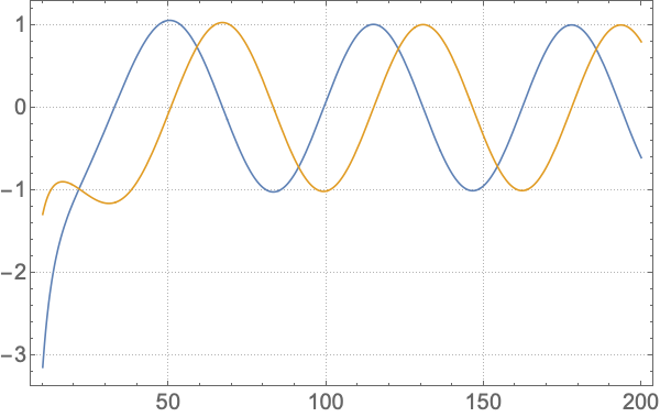
RW = ReggeWheelerRadial[2, 2, 0.1, Method -> {"NumericalIntegration", "Domain" -> {10, 10^4}}, "BoundaryConditions" -> "Up"]
for the “Up” solution. Note you have to set the integration “Domain”. The resulting ReggeWheelerRadialFunction can be rapidly evaluated (though this method is not as effective for beyond machine precision results).
You can plot the real and imaginary parts of the above radial solution using Plot[RW[r] // ReIm // Evaluate, {r, 10, 200}, PlotTheme -> "Detailed",
PlotLegends -> None, BaseStyle -> 20]. This gives:
Authors and contributors
David Q. Aruquipa, Marc Casals, Leanne Durkan, Jonathan Thompson, Niels Warburton, Barry Wardell