SpinWeightedSpheroidalHarmonics

The SpinWeightedSpheroidalHarmonics package for Mathematica provides functions for computing spin-weighted spheroidal harmonics, spin-weighted spherical harmonics, and their associated eigenvalues. Support is included for both arbitrary-precision numerical evaluation and for series expansions.

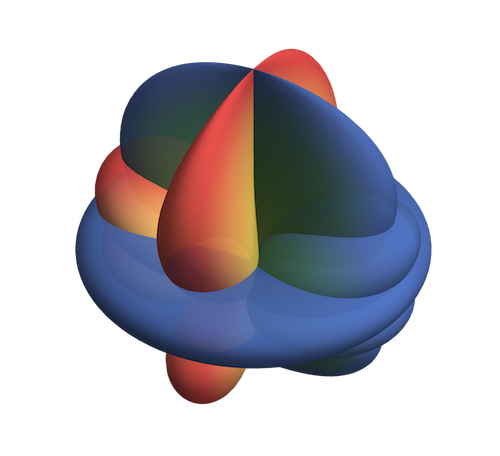
Explicitly the package computes solutions to the equation

where

$S$ is the spin-weighted spheroidal harmonic
$s$ is the spin-weight
$l,m$ are the multipolar indices
$\gamma$ is the spheroidicity
$\lambda$ is the spheroidal eigenvalue

Examples

Numerical evaluation

Evaluating the spheroidal eigenfunction for $s=-2$, $l=2$, $m=2$, $\gamma=1.5$, $\theta = \pi/2$, $\phi=0$ is done via

In  := SpinWeightedSpheroidalHarmonicS[-2, 2, 2, 1.5`30][π/2, 0]
Out := 0.066929509191705738197645539

Likewise the corresponding eigenvalue, $\lambda$, is computed by

In  := SpinWeightedSpheroidalEigenvalue[-2, 2, 2, 1.5`30]
Out := -5.5776273646788261891028539326

Note the output tracks the precision of the input so it is very easy to compute high precision results.

Small frequency expansions

Small frequency expansions can be performed for the eigenfunctions and eigenvalues

For given $s,l,m$ the eigenfunction can be expanded via, e.g.,

Series[SpinWeightedSpheroidalHarmonicS[2, 3, 2, γ][θ,ϕ], {γ, 0, 1}]

This returns

$\frac{1}{2} \sqrt{\frac{7}{\pi }} e^{2 i \phi } \sin^4\left(\frac{\theta }{2}\right) (3 \cos (\theta)+2)-\frac{1}{72} \gamma \left(\sqrt{\frac{7}{\pi }}e^{2 i \phi } \sin ^4\left(\frac{\theta }{2}\right)(54 \cos (\theta )+27 \cos (2 \theta)+29)\right)+O\left(\gamma ^2\right)$

The series expansion above can also be performed for generic values of $s,l,m$ which returns a series in SpinWeightedSphericalHarmonicsY functions.

For generic $s,l,m$ the eigenvalues are expanded via:

Series[SpinWeightedSpheroidalEigenvalue[s, l, m, γ], {γ, 0, 1}]

returns

$\left(l^2+l-s (s+1)\right) + \gamma \left(-\frac{2 m s^2}{l (l+1)}-2 m\right) + O\left(\gamma ^2\right).$

The code is fast but note that in general the series expansion will be quicker to compute if when explicit values of $s$, $l$, $m$ are provided.

High frequency expansions

It is also possible to calculate series expansions of the eigenvalue about $\gamma = \infty$. For example, for the $s=2,l=2,m=2$ case, the command:

Series[SpinWeightedSpheroidalEigenvalue[2, 2, 2, γ], {γ, ∞, 6}]

returns

$-6 \gamma -1 + \frac{3}{4 \gamma } -\frac{15}{64 \gamma ^3} -\frac{3}{16 \gamma ^4} +\frac{3}{512 \gamma ^5} + \frac{27}{128 \gamma ^6} +O\left[\frac{1}{\gamma}\right]^7$

Currently, the high frequency expansions require explicit values for $s,l,m$.

Further examples

See the Mathematica Documentation Centre for a tutorial and documentation on individual functions.

Citing

In addition to acknowledging the Black Hole Perturbation Toolkit as suggested on the front page we also recommend citing the specific package version you use via the citation information on the package’s Zenodo page linked from the above DOI.

Authors and contributors

Barry Wardell, Niels Warburton, Kwinten Fransen, Samuel Upton, Kevin Cunningham, Marc Casals, Sarp Akcay, Adrian Ottewill