WaSABI

Overview

WaSABI (Waveform Simulations of Asymmetric Binary Inspirals) is a Mathematica package for generating gravitational waveforms from self-force (SF) theory and from SF–post-Newtonian (PN) hybrids. The currently available models are for quasicircular inspirals.

Self-force models:

• 1PAT1ea and 1PAT1R: two first-post-adiabatic (1PA) models for spinning binaries, where the primary black hole is slowly rotating.
• 1PAT1: a 1PA model for non-spinning binaries.
• 0PAKerr: an adiabatic inspiral model for spinning binaries.
• 0PASchwarz: an adiabatic inspiral model for non-spinning binaries.

Self-force/post-Newtonian hybrids:

• WaSABI-C: an SF+PN hybrid for spin (anti-)aligned spinning binaries.
• WaSABI-C_v0.9: an SF+PN hybrid with a spinning primary and a non-spinning secondary.

Each model evolves a set of coupled first-order ODEs through phase space and combines the resulting trajectory with mode amplitudes to produce the waveform. For fast EMRI waveforms in Python see FastEMRIWaveforms.

Installation

WaSABI is distributed as a paclet (the model data are included). Once the BHPToolkit paclet server is set up (see Get started), install it by name:

PacletSiteRegister["https://pacletserver.bhptoolkit.org", "Black Hole Perturbation Toolkit Paclet Server"]
PacletSiteUpdate["https://pacletserver.bhptoolkit.org"]
PacletInstall["WaSABI"]

Usage

Loading the package

<< WaSABI`

Getting information about a model

List the implemented models with:

ListModels[]

{"0PAKerr", "0PASchwarz", "1PAT1ea", "1PAT1", "1PAT1R", "WaSABI-C", "WaSABI-C_v0.9"}

Say you want to generate a gravitational waveform with the model 1PAT1. You can query the initial conditions that this model requires using:

InitialConditions["1PAT1"]

<|"M" -> _, "r0" -> _, "\[Nu]" -> _, "\[Phi]" -> _|>

You can query which $(\ell, \lvert m\rvert)$ modes are available using ListModes:

ListModes["1PAT1"]

{"(2,1)", "(2,2)", "(3,1)", "(3,2)", "(3,3)", "(4,1)", "(4,2)", "(4,3)", "(4,4)", "(5,1)", "(5,2)", "(5,3)", "(5,4)", "(5,5)"}

Before using a model you will probably want to read how it was constructed. CiteModel returns the BibTeX for the article(s) in which the model was developed:

CiteModel["1PAT1"]

@article{Wardell:2021fyy,
    author = "Wardell, Barry and Pound, Adam and Warburton, Niels and Miller, Jeremy and Durkan, Leanne and Le Tiec, Alexandre",
    title = "{Gravitational Waveforms for Compact Binaries from Second-Order Self-Force Theory}",
    eprint = "2112.12265",
    archivePrefix = "arXiv",
    primaryClass = "gr-qc",
    doi = "10.1103/PhysRevLett.130.241402",
    journal = "Phys. Rev. Lett.",
    volume = "130",
    number = "24",
    pages = "241402",
    year = "2023"
}

Generating a waveform

BinaryInspiral generates a BinaryInspiralModel object that stores the waveform and the phase-space trajectory for a given set of initial conditions. The model is chosen with the "Model" option (default "1PAT1"):

inspiral = BinaryInspiral[<|"r0" -> 10, "M" -> 1, "\[Nu]" -> 1/10, "\[Phi]" -> 0|>, "Model" -> "1PAT1"];

Keys[inspiral] lists its properties: "Model", "InitialConditions", "Duration", "Waveform" and "Trajectory". BinaryInspiral also accepts "Precision", "Accuracy" and "StopCondition" options.

The forcing functions

The models are built by evolving a set of first-order coupled ODEs through phase space. For a set of parameters $x_i$, the evolution equations are $\dot{x}_i(t)=F_{x_i}(x_j(t))$, where the functions $F_{x_i}$ are called the forcing functions. To diagnose the dynamics, call ForcingTerms:

FT = ForcingTerms["1PAT1"]

This object represents the set of forcing functions of the model 1PAT1. It is a function on phase space, and it can be evaluated at a particular point in parameter space with:

FT[<|"r0" -> 10, "\[Phi]" -> 0, "\[Nu]" -> 0.1, "M" -> 1|>]

<|"d\[CapitalOmega]/dt" -> 7.86312*10^-6, "d\[Phi]/dt" -> 0.0316228, "d\[Nu]/dt" -> 0., "dM/dt" -> 0.|>

Examples

Plotting the waveform and trajectory

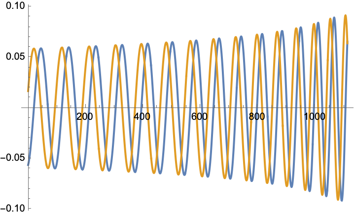
Plot the $\ell=2$, $m=2$ mode of the gravitational waveform for the inspiral generated above:

tmax = inspiral["Duration"];
Plot[Evaluate[ReIm[inspiral["Waveform"][2, 2][t]]], {t, 0, tmax}]

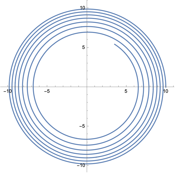
Plot the orbital trajectory:

r0 = inspiral["Trajectory"]["r0"];
\[Phi] = inspiral["Trajectory"]["\[Phi]"];
ParametricPlot[{r0[t] Cos[\[Phi][t]], r0[t] Sin[\[Phi][t]]}, {t, 0, tmax}]

Comparing forcing functions

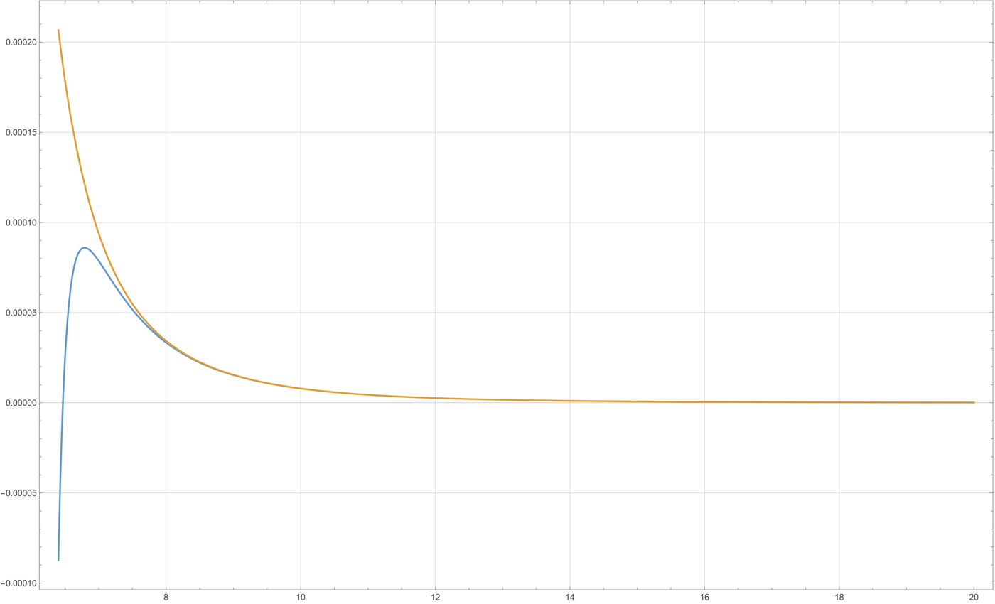
Plot the forcing term $d\Omega/dt$ of 1PAT1 as a function of the orbital separation $r_0$, and compare it with the corresponding forcing term of the hybrid model WaSABI-C:

FT1PA = ForcingTerms["1PAT1"];
FTHyb = ForcingTerms["WaSABI-C"];

Plot[{
  FT1PA[<|"r0" -> r, "\[Phi]" -> 0, "\[Nu]" -> 0.1, "M" -> 1|>][["d\[CapitalOmega]/dt"]],
  FTHyb[<|"\[Omega]" -> 1/r^(3/2), "\[Phi]" -> 0, "\[Nu]" -> 0.1, "M" -> 1, "\[Chi]1" -> 10^-5, "\[Chi]2" -> 0., "\[Delta]m" -> 0, "\[Delta]\[Nu]" -> 0, "\[Delta]\[Chi]" -> 0|>][["d\[Omega]/dt"]]
  }, {r, 20, 6.4}, PlotRange -> All, GridLines -> Automatic, Frame -> True]

Model references

In addition to the citations below, please make sure you cite the original authors of any model you use. You can retrieve the relevant BibTeX with CiteModel, e.g. CiteModel["1PAT1"] as shown above.

Authors and contributors

Barry Wardell, Josh Mathews, Loïc Honet

Citing WaSABI

If you use WaSABI in your research, please acknowledge the Toolkit:

WaSABI also requests the following citations:

• WaSABI
  BibTeX

  @software{BHPToolkit:WaSABI,
    author       = {Wardell, Barry and Mathews, Josh and Honet, Loïc},
    title        = {WaSABI},
    month        = jan,
    year         = 2026,
    publisher    = {Zenodo},
    version      = {1.1.3},
    doi          = {10.5281/zenodo.18268703},
    url          = {https://doi.org/10.5281/zenodo.18268703},
  }

• Black Hole Perturbation Toolkit
  BibTeX

  @misc{BHPToolkit,
    title = {{Black Hole Perturbation Toolkit}},
    howpublished = {(\href{http://bhptoolkit.org/}{bhptoolkit.org})},
  }

See how to cite for further guidance.