ReggeWheeler

Overview

The ReggeWheeler package for Mathematica computes solutions to the Regge–Wheeler equation, which governs perturbations of the Schwarzschild spacetime:

where the potential is given by

and $f = 1-2M/r$, a prime denotes differentiation with respect to $r$, $M$ is the black hole mass, $\omega$ is the mode frequency, $\Psi$ is the Regge–Wheeler master variable and $\mathcal{T}$ is the source.

The package provides:

• homogeneous “In” and “Up” solutions and their asymptotic amplitudes, computed with the semi-analytic MST method, direct numerical integration, or Mathematica’s HeunC function;
• solutions of the Zerilli equation (for $\lvert s\rvert = 2$) as well as the Regge–Wheeler equation, and static ($\omega = 0$) modes;
• inhomogeneous solutions and energy and angular-momentum fluxes for a point particle on a circular geodesic orbit, including (in the development version) a hyperboloidal spectral method.

The package depends on the SpinWeightedSpheroidalHarmonics and KerrGeodesics packages. For perturbations of Kerr spacetime see the Teukolsky package.

Installation

ReggeWheeler is distributed as a paclet. Once the BHPToolkit paclet server is set up (see Get started), install it together with its dependencies:

PacletSiteRegister["https://pacletserver.bhptoolkit.org", "Black Hole Perturbation Toolkit Paclet Server"]
PacletSiteUpdate["https://pacletserver.bhptoolkit.org"]
PacletInstall["SpinWeightedSpheroidalHarmonics"]
PacletInstall["KerrGeodesics"]
PacletInstall["ReggeWheeler"]

Usage

Loading the package

<< ReggeWheeler`

Point-particle modes and fluxes

The source is implemented for a point particle moving on a circular geodesic orbit. For example, the $\ell=2$, $m=2$ mode for a particle at orbital radius $r_0 = 10M$ is computed with ReggeWheelerPointParticleMode[s, l, m, n, orbit]:

r0 = 10`30;
orbit = KerrGeoOrbit[0, r0, 0, 1];

s = 2; l = 2; m = 2; n = 0;
mode = ReggeWheelerPointParticleMode[s, l, m, n, orbit];

mode is a ReggeWheelerMode object which can be queried for results. The energy and angular momentum fluxes at infinity ($\mathcal{I}$) and the horizon ($\mathcal{H}$) are given by mode["Fluxes"]:

mode["Fluxes"]
(* <|"Energy" -> <|"I" -> 0.000026843977395510576377, "H" -> 5.6541387345369358451*10^-9|>,
     "AngularMomentum" -> <|"I" -> 0.00084888110027888050954, "H" -> 1.78799566077188627708*10^-7|>|> *)

Note the high precision of the input value of $r_0$. This is required by default, as the package uses the MST method to calculate the homogeneous solutions. You can also extract "EnergyFlux", "AngularMomentumFlux", "s", "l", "m", "ω", "Eigenvalue", "RadialFunctions", "AngularFunction", "Amplitudes" and "Method" from a ReggeWheelerMode.

For even-parity modes ($\ell + m$ even) the radial functions are computed from the Zerilli equation, and for odd-parity modes from the Regge–Wheeler equation.

Homogeneous solutions

The homogeneous radial solutions alone are computed with ReggeWheelerRadial[s, l, ω], which returns an association of ReggeWheelerRadialFunctions (or a single one if only one boundary condition is requested). A ReggeWheelerRadialFunction can be evaluated at a radius r, and queried for properties such as "Amplitudes" (incidence, transmission and reflection) and "Eigenvalue".

The following options are available:

• "BoundaryConditions" — {"In", "Up"} (default), "In" or "Up".
• "Potential" — "ReggeWheeler" (default) or "Zerilli" (only for $\lvert s\rvert = 2$).
• Method — "MST" (default), "NumericalIntegration" or "HeunC", described below.
• WorkingPrecision, PrecisionGoal, AccuracyGoal — by default set from the precision of $\omega$.

MST

The default method uses the semi-analytic Mano–Suzuki–Takasugi (MST) expansion. It works well for high-precision results, but currently needs high-precision input (a warning is given for machine-precision input), and is slower to evaluate than numerical integration. Use it explicitly by passing Method -> "MST". By default both the “In” and “Up” solutions are computed; use, e.g., "BoundaryConditions" -> "Up" to compute only one.

Numerical integration

The numerical integration method is used via, e.g.,

RW = ReggeWheelerRadial[2, 2, 0.1, Method -> {"NumericalIntegration", "Domain" -> {10, 10^4}}, "BoundaryConditions" -> "Up"]

for the “Up” solution. Note that you have to set the integration "Domain". The resulting ReggeWheelerRadialFunction can be evaluated rapidly, though this method is not as effective for results beyond machine precision.

HeunC

With Mathematica 12.1 or newer, Method -> "HeunC" computes the solutions using Mathematica’s built-in confluent Heun function.

Hyperboloidal method

For circular equatorial orbits, ReggeWheelerPointParticleMode can alternatively solve the Regge–Wheeler–Zerilli equations with a hyperboloidal compactification and a spectral method (arXiv:2202.01794, arXiv:2411.14976):

orbit = KerrGeoOrbit[0, 10`30, 0, 1];
mode = ReggeWheelerPointParticleMode[2, 2, 2, 0, orbit, Method -> "Hyperboloidal"];
mode["Fluxes"]

This method currently supports $s=2$ and $n=0$ only. The number of grid points can be set with Method -> {"Hyperboloidal", "GridPoints" -> N}. The hyperboloidal method was added after the 0.3.0 release, so it currently requires the development version of the package from the GitHub repository.

Examples

Plotting a radial solution

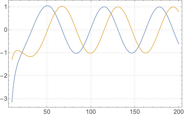
Plot the real and imaginary parts of the numerically integrated “Up” solution computed above:

Plot[RW[r] // ReIm // Evaluate, {r, 10, 200}, PlotTheme -> "Detailed", PlotLegends -> None, BaseStyle -> 20]

Further examples using the Toolkit’s Mathematica packages can be found in the Mathematica Toolkit Examples repository.

Authors and contributors

David Q. Aruquipa, Marc Casals, William Doherty, Leanne Durkan, Josh Mathews, Adrian Ottewill, Jonathan Thompson, Niels Warburton, Barry Wardell

Citing ReggeWheeler

If you use ReggeWheeler in your research, please acknowledge the Toolkit:

ReggeWheeler also requests the following citations:

• ReggeWheeler
  BibTeX

  @software{BHPToolkit:ReggeWheeler,
    author       = {Wardell, Barry and Warburton, Niels and Thompson, Jonathan},
    title        = {ReggeWheeler},
    month        = sep,
    year         = 2020,
    publisher    = {Zenodo},
    version      = {0.3.0},
    doi          = {10.5281/zenodo.17417009},
    url          = {https://doi.org/10.5281/zenodo.17417009},
  }

• For use of the hyperboloidal method:
  Panosso Macedo et al., Hyperboloidal method for frequency-domain self-force calculations, Phys. Rev. D 105, 104033 (2022) arXiv Inspire
  BibTeX

  @article{PanossoMacedo:2022fdi,
      author = "Panosso Macedo, Rodrigo and Leather, Benjamin and Warburton, Niels and Wardell, Barry and Zengino{\u{g}}lu, An{\i}l",
      title = "{Hyperboloidal method for frequency-domain self-force calculations}",
      eprint = "2202.01794",
      archivePrefix = "arXiv",
      primaryClass = "gr-qc",
      doi = "10.1103/PhysRevD.105.104033",
      journal = "Phys. Rev. D",
      volume = "105",
      number = "10",
      pages = "104033",
      year = "2022"
  }

• Leather, Gravitational self-force with hyperboloidal slicing and spectral methods, Gen. Rel. Grav. 57, 112 (2025) arXiv Inspire
  BibTeX

  @article{Leather:2024mls,
      author = "Leather, Benjamin",
      title = "{Gravitational self-force with hyperboloidal slicing and spectral methods}",
      eprint = "2411.14976",
      archivePrefix = "arXiv",
      primaryClass = "gr-qc",
      doi = "10.1007/s10714-025-03443-9",
      journal = "Gen. Rel. Grav.",
      volume = "57",
      number = "7",
      pages = "112",
      year = "2025"
  }

• Black Hole Perturbation Toolkit
  BibTeX

  @misc{BHPToolkit,
    title = {{Black Hole Perturbation Toolkit}},
    howpublished = {(\href{http://bhptoolkit.org/}{bhptoolkit.org})},
  }

See how to cite for further guidance.