KerrGeoPy

Overview

KerrGeoPy is a Python implementation of the Toolkit’s KerrGeodesics Mathematica package. It computes bound timelike geodesics in Kerr spacetime and is intended for computing orbital trajectories for extreme mass-ratio inspirals (EMRIs).

It implements the analytical solutions for stable bound orbits from Fujita and Hikida and for plunging orbits from Dyson and van de Meent. It also provides functions for constants of motion (energy, angular momentum, Carter constant), orbital frequencies in Mino time and Boyer–Lindquist time, the separatrix, and conversions to physical units, and it can plot and animate orbits.

Orbit parametrization

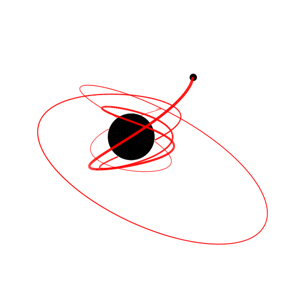
Orbits are computed in Boyer–Lindquist coordinates $(t,r,\theta,\phi)$ in geometrized units ($G=c=1$). With $M$ the mass of the primary and $J$ its angular momentum, stable bound orbits are parametrized by the spin $a$, semi-latus rectum $p$, eccentricity $e$ and the cosine of the inclination $x$:

$a$ and $x$ lie between $-1$ and $1$ and $e$ between $0$ and $1$. Retrograde orbits are represented by a negative value of $a$ or $x$. Polar orbits, marginally bound orbits and orbits about an extremal Kerr black hole are not supported.

Constants of motion are dimensionless and scale-invariant, normalized by the primary mass $M$ and the secondary mass $\mu$:

Plunging orbits are parametrized by $(a, \mathcal{E}, \mathcal{L}, \mathcal{Q})$.

Installation

Install from PyPI:

pip install kerrgeopy

or from conda-forge:

conda install -c conda-forge kerrgeopy

KerrGeoPy uses functions introduced in scipy 1.8, so you may need to update scipy with pip install scipy -U (pip usually does this automatically). Some plotting and animation functions use features from matplotlib 3.7 and need ffmpeg, which is available from Homebrew or conda-forge.

Usage

Stable bound orbits

Construct a StableOrbit from $(a, p, e, x)$. The trajectory() method returns the components $t(\lambda)$, $r(\lambda)$, $\theta(\lambda)$, $\phi(\lambda)$ as functions of Mino time $\lambda$:

import kerrgeopy as kg
from math import cos, pi
import numpy as np

orbit = kg.StableOrbit(0.999, 3, 0.4, cos(pi/6))

t, r, theta, phi = orbit.trajectory()

time = np.linspace(0, 20, 200)
r(time)

By default $t$ and $r$ are dimensionless (normalized by $M$). orbit.plot(0, 10) draws the orbit from $\lambda = 0$ to $\lambda = 10$.

Orbital properties

E, L, Q = orbit.constants_of_motion()

upsilon_r, upsilon_theta, upsilon_phi, gamma = orbit.mino_frequencies()

omega_r, omega_theta, omega_phi = orbit.fundamental_frequencies()

For the orbit above, the KerrGeoPy README gives $\mathcal{E} = 0.877$, $\mathcal{L} = 1.903$, $\mathcal{Q} = 1.265$ and $\Omega_r = 0.056$, $\Omega_\theta = 0.109$, $\Omega_\phi = 0.152$ (to three decimal places).

These quantities are dimensionless by default. If you pass the masses M and mu (in solar masses) to StableOrbit, you can request physical units, for example orbit.fundamental_frequencies(units="mHz") or orbit.trajectory(distance_units="km", time_units="days").

Plunging orbits

Construct a PlungingOrbit from $(a, \mathcal{E}, \mathcal{L}, \mathcal{Q})$:

orbit = kg.PlungingOrbit(0.9, 0.94, 0.1, 12)
t, r, theta, phi = orbit.trajectory()

Alternative parametrizations

Build a StableOrbit from the spin and constants of motion $(a, \mathcal{E}, \mathcal{L}, \mathcal{Q})$:

orbit = kg.StableOrbit.from_constants(0.9, 0.95, 1.6, 8)

or build a generic Orbit from the spin, an initial position $(t_0,r_0,\theta_0,\phi_0)$ and an initial four-velocity $(u^t_0,u^r_0,u^\theta_0,u^\phi_0)$:

stable_orbit = kg.StableOrbit(0.999, 3, 0.4, cos(pi/6))

x0 = stable_orbit.initial_position
u0 = stable_orbit.initial_velocity

orbit = kg.Orbit(0.999, x0, u0)

Graphics

plot() returns a matplotlib figure and axes. animate(filename, ...) saves an mp4 animation of the orbit. It needs ffmpeg and can take several minutes to run.

Examples

The KerrGeoPy documentation has tutorial notebooks (Getting Started, Orbital Properties, Trajectory, Graphics) and a full API reference. The notebooks are also in the docs/source/notebooks folder of the repository.

Authors and contributors

Seyong Park, Zachary Nasipak

Citing KerrGeoPy

If you use KerrGeoPy in your research, please acknowledge the Toolkit:

KerrGeoPy also requests the following citation:

• KerrGeoPy: A Python Package for Computing Timelike Geodesics in Kerr Spacetime, J. Open Source Softw. 9, 6587 (2024) arXiv Inspire
  BibTeX

  @article{Park:2024sjj,
      author = "Park, Seyong and Nasipak, Zachary",
      title = "{KerrGeoPy: A Python Package for Computing Timelike Geodesics in Kerr Spacetime}",
      eprint = "2406.01413",
      archivePrefix = "arXiv",
      primaryClass = "gr-qc",
      doi = "10.21105/joss.06587",
      journal = "J. Open Source Softw.",
      volume = "9",
      number = "98",
      pages = "6587",
      year = "2024"
  }

See how to cite for further guidance.