Fast post-adiabatic waveforms in FEW

In this tutorial we outline the basic features of the FEW implementation of 1PAT1R, a post-adiabatic self-force waveform model describing the quasicircular inspiral of a spinning secondary object (black hole or neutron star) into a slowly spinning Kerr black hole. Both spins are assumed to be aligned with the orbital angular momentum.

We adopt the following notational conventions:

• The initial masses of the objects are denoted \(m_1\) and \(m_2\), with \(m_1 > m_2\).

• The initial total mass is \(M := m_1 + m_2\), and the symmetric mass ratio is \(\nu := \frac{m_1m_2}{(m_1+m_2)^2}\).

• The initial dimensionless spin parameters of the two components are denoted \(\chi_1\) and \(\chi_2\).

• The orbital radius is parameterised by \(p(t) := [M\Omega_{\rm phys}(t)]^{-2/3}\), where \(\Omega_{\rm phys}(t)\) is the physical orbital frequency.

The model is subject to the following parameter restrictions:

	\(m_2\)	\(\chi_1\)	\(\chi_2\)	\(p\)
Allowed	\((0, m_1]\)	\([-1, 1]\)	\([-1, 1]\)	\({\rm max}(p_{\rm ISCO}+0.01, 6.26) \leq p \leq 30\)
Recommended	—	\(\|\chi_1\| < 25\nu\)	\(\|\chi_2\| \ll \nu^{-1}\)	\(6 + 1.5\nu^{1/4} < p < 0.02\nu^{-2}\)

where \(p_{\rm ISCO}\) is the radius of the innermost stable circular orbit (divided by \(m_1\)) for a Kerr black hole of mass \(m_1\) and dimensionless spin \(\chi_1\).

import numpy as np
import matplotlib.pyplot as plt

1. Waveform generation

1.1. Generic waveform interface

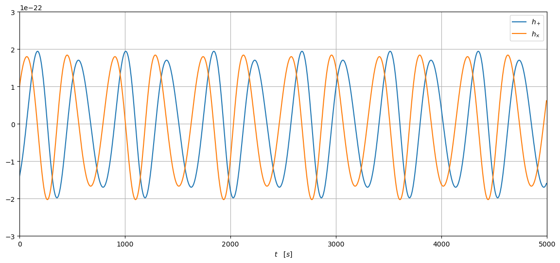
1PAT1R waveforms can be generated using the generic GenerateEMRIWaveform waveform generator. For detector frame waveforms, a generator can be instantiated as follows:

from few.waveform import GenerateEMRIWaveform

inspiral_kwargs = {}
amplitude_kwargs = {}

waveform_generator = GenerateEMRIWaveform(
        "Circ1PAT1R",
        #sum_kwargs = dict(pad_output=True),
        inspiral_kwargs = inspiral_kwargs,
        amplitude_kwargs = amplitude_kwargs,
        frame = "detector"
    )

We now consider the system with the following parameters:

# Define parameters
m1 = 1e6        # primary mass [solar masses]
m2 = 10         # secondary mass [solar masses]
chi1  = 1e-5    # primary spin chi1 (dimensionless)
p0 = 9.0        # initial orbital separation [M]
chi2  = 0.1     # secondary spin

dL = 1.0        # luminosity distance [Gpc]
e0 = 0.0        # eccentricity
xI0 = 1.0       # cos(inclination)

qK = np.pi/3    # initial BH spin polar angle in ecliptic coords [rad]
phiK = np.pi/4  # initial BH spin azimuthal angle in ecliptic coords [rad]
qS = np.pi/5    # sky location polar angle in ecliptic coords [rad]
phiS = np.pi/3  # sky location azimuthal angle in ecliptic coords [rad]

Phi_phi0 = np.pi/4      # initial azimuthal phase [rad]
Phi_theta0 = np.pi/4    # initial polar phase [rad] (redundant for this model)
Phi_r0 = np.pi/4        # initial radial phase [rad] (redundant for this model)

dt = 5.         # time step for the returned waveform [s]
T  = 1          # total duration [yr]

params = [m1, m2, chi1, p0, e0, xI0, dL, qS, phiS, qK, phiK, Phi_phi0, Phi_theta0, Phi_r0, chi2]

The waveform can be generated as follows.

h = waveform_generator(*params, T=T, dt=dt)
time_array = np.arange(0, len(h)) * dt

plt.gcf().set_size_inches(14, 6)
plt.plot(time_array[:1000], h.real[:1000], label=r"$h_+$")
plt.plot(time_array[:1000], -h.imag[:1000], label=r"$h_{\times}$")
plt.xlim(0, 5000)
plt.ylim(-3e-22, 3e-22)
plt.xlabel(r"$t \quad [s]$")
plt.legend()
plt.grid()

1.2. Waveform class

One can directly instantiate a 1PAT1R waveform generator object:

from few.waveform import Circ1PAT1R

WF1PAT1R = Circ1PAT1R()

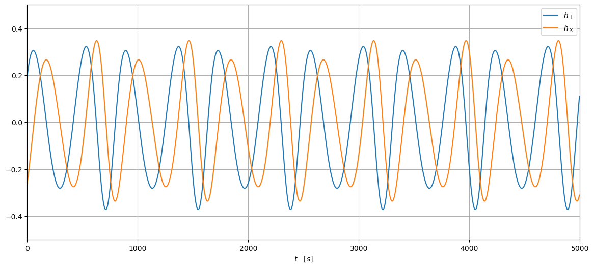
To generate a source-frame waveform with given parameters, simply call

theta = phi = np.pi/4 # polar and azimuthal viewing angles [rad]
h_src = WF1PAT1R(m1, m2, chi1, p0, theta, phi, chi2, dt=dt, T=T)
time_array = dt*np.arange(0, len(h_src))

plt.gcf().set_size_inches(14, 6)
plt.plot(time_array[:1000], h_src[:1000].real,  label=r"$h_+$")
plt.plot(time_array[:1000],-h_src[:1000].imag,  label=r"$h_\times$")
plt.ylim(-0.5, 0.5)
plt.xlim(0, 5000)
plt.xlabel(r"$t \quad[s]$")
plt.legend()
plt.grid()

2. Post-adiabatic trajectories

from few.trajectory.inspiral import EMRIInspiral
from few.trajectory.ode.circ1pat1r import TrajectoryCirc1PAT1R

In this section we describe the implementation of the post-adiabatic trajectory. We highlight the following features:

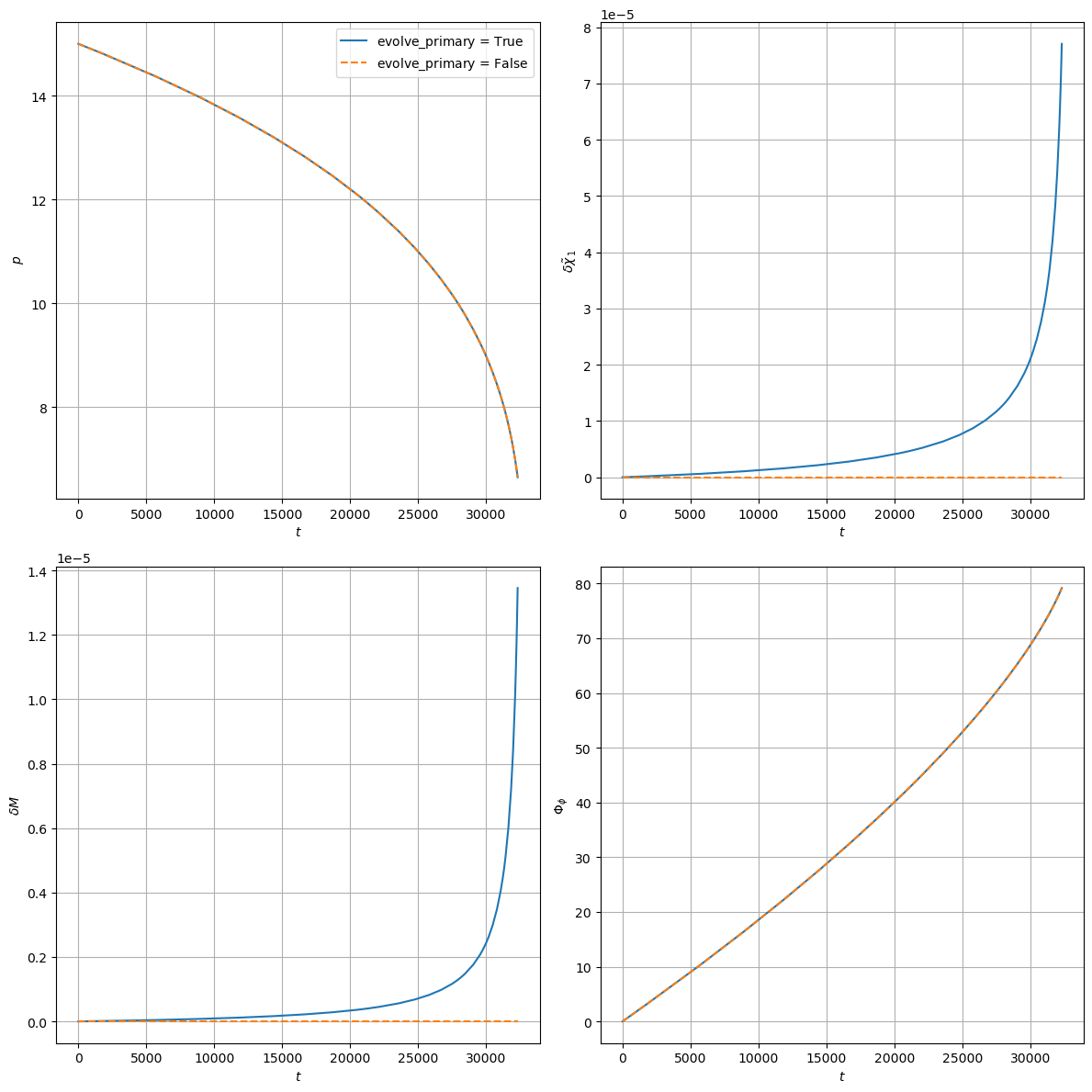
• The model incorporates the evolution of the primary black hole’s mass due to the emission of gravitational radiation. Internally this is described using the mass deviation parameter

  \[\delta M(t) := \frac{m_1^{\rm phys}(t) - m_1}{\nu M}, \qquad\qquad (2.1)\]

  where \(m_1^{\rm phys}(t)\) is the time-varying physical mass of the primary black hole.

• The model additionally incorporates the evolution of the primary black hole’s spin, but the secondary object’s spin is treated as fixed. Internally, we make use of the rescaled variables \(\tilde \chi_1\) and \(\tilde \chi_2\) defined by

  \[\tilde\chi_1 := \frac{m_1}{M}\chi_1 = \frac{1}{2}(1+\sqrt{1-4\nu})\chi_1, \qquad\tilde\chi_2 := \frac{m_2}{M}\chi_2 = \frac{1}{2}(1-\sqrt{1-4\nu})\chi_2. \qquad\qquad (2.2)\]

  The evolution of the primary spin is then described using the parameter \(\delta\tilde\chi_1(t) := \tilde\chi_1(t) - \tilde\chi_1(t=0)\).

Altogether the trajectory state vector for this model is \(\vec y = (p, e, x_I, \Phi_\phi, \Phi_\theta, \Phi_r, \delta M, \delta\tilde\chi_1)\), where the first 6 elements are the same as for the adiabatic order models included in FEW.

The system of ODEs describing the time-evolution of the state vector is defined using the TrajectoryCirc1PAT1R class. These differential equations can be integrated using the generic EMRIInspiral solver:

# Instantiate integrator
traj = EMRIInspiral(func=TrajectoryCirc1PAT1R)

# System parameters
m1 = 1e6       # primary mass [solar masses]
m2 = 1e6       # secondary mass [solar masses]
a  = -0.2       # primary spin chi1 (dimensionless)
chi2  = -0.1   # secondary spin
p0 = 15.0      # initial orbital separation [M]
dt = 1.   # time step [s]
T  = 1    # total duration [yr]

# Integrate
t, p, e, x, Phi_phi, Phi_theta, Phi_r, deltaM, deltachit1 = traj(
    m1, m2,
    a,        # chi1 (primary spin)
    p0,
    0.0,      # e0: circular
    1.0,      # xI: equatorial prograde
    chi2,
    T=T
)

plt.gcf().set_size_inches(12, 12)
plt.subplot(221)
plt.plot(t, p)
plt.xlabel(r"$t$")
plt.ylabel(r" $p$")
plt.grid()

plt.subplot(222)
plt.plot(t, deltachit1)
plt.xlabel(r"$t \quad [s]$")
plt.ylabel(r"$\delta\tilde\chi_1$")
plt.grid()

plt.subplot(223)
plt.plot(t, deltaM)
plt.xlabel(r"$t \quad [s]$")
plt.ylabel(r"$\delta M$")
plt.grid()

plt.subplot(224)
plt.plot(t, Phi_phi)
plt.xlabel(r"$t$")
plt.ylabel(r"$\Phi_\phi$")
plt.grid()

plt.gcf().tight_layout()

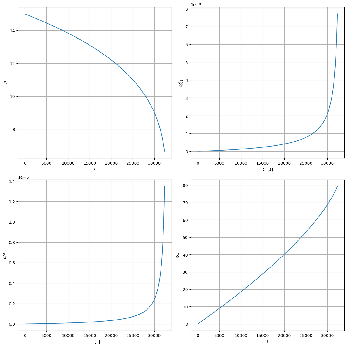
Note that the trajectory evolves the parameters \(\delta M\) and \(\delta \tilde\chi_1\) by default. This can be switched off by setting evolve_primary = False when instantiating the trajectory class (it can also be set through inspiral_kwargs in GenerateEMRIWaveform – see Sec. 4):

traj_no_evolve_primary = EMRIInspiral(func=TrajectoryCirc1PAT1R, evolve_primary=False)

t_2, p_2, e_2, x_2, Phi_phi_2, Phi_theta_2, Phi_r_2, deltaM_2, deltachit1_2 = traj_no_evolve_primary(
    m1, m2,
    a,        # chi1 (primary spin)
    p0,
    0.0,      # e0: circular
    1.0,      # xI: equatorial prograde
    chi2,
    T=T
)

plt.gcf().set_size_inches(12, 12)
plt.subplot(221)
plt.plot(t, p, label=r"$\text{evolve\_primary = True}$")
plt.plot(t_2, p_2, ls='--', label=r"$\text{evolve\_primary = False}$")
plt.xlabel(r"$t$")
plt.ylabel(r" $p$")
plt.grid()
plt.legend()

plt.subplot(222)
plt.plot(t, deltachit1, label=r"$\text{evolve\_primary = True}$")
plt.plot(t_2, deltachit1_2, ls='--', label=r"$\text{evolve\_primary = False}$")
plt.xlabel(r"$t$")
plt.ylabel(r"$\delta\tilde\chi_1$")
plt.grid()

plt.subplot(223)
plt.plot(t, deltaM, label=r"$\text{evolve\_primary = True}$")
plt.plot(t_2, deltaM_2, ls='--', label=r"$\text{evolve\_primary = False}$")
plt.xlabel(r"$t$")
plt.ylabel(r"$\delta M$")
plt.grid()

plt.subplot(224)
plt.plot(t, Phi_phi, label=r"$\text{evolve\_primary = True}$")
plt.plot(t_2, Phi_phi_2, ls='--', label=r"$\text{evolve\_primary = False}$")
plt.xlabel(r"$t$")
plt.ylabel(r"$\Phi_\phi$")
plt.grid()

plt.gcf().tight_layout()

3. Post-adiabatic waveform amplitudes

from few.amplitude.ampinterp1d import AmplitudeCirc1PAT1R

The full waveform mode amplitude \(\mathcal{A}_{\ell m}\) in 1PAT1R is given by

\[\begin{split}\begin{aligned} \mathcal{A}_{\ell m} = \Delta_m(\nu)\Big[&\mathcal{A}^{\rm 0PA}_{\ell m}(p) + \nu\bar{\mathcal{A}}^{\rm 1PA}_{\ell m}(p) \\ & \qquad + \tilde\chi_1\mathcal{A}^{\rm 1PA\chi_1}_{\ell m}(p) + \tilde\chi_2\mathcal{A}^{\rm 1PA\chi_2}_{\ell m}(p) + \nu\,\delta M\,\mathcal{A}^{\rm 1PA\delta M}_{\ell m}(p)\Big] \end{aligned} \qquad (3.1)\end{split}\]

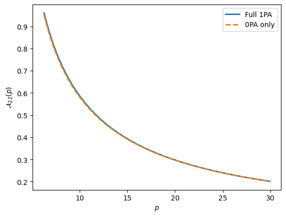
where \(\mathcal{A}_{\ell m}^{\rm 0PA}\) and \(\nu\bar{\mathcal{A}}_{\ell m}^{\rm 1PA}\) are the non-spinning 0PA and 1PA self-force amplitudes, \(\tilde\chi_1\mathcal{A}_{\ell m}^{\rm 1PA\chi_1}\) and \(\tilde\chi_2\mathcal{A}_{\ell m}^{\rm 1PA\chi_2}\) are the corrections due to the primary and secondary spin, respectively, and \(\nu\delta M\mathcal{A}_{\ell m}^{\rm 1PA\delta M}\) is a correction due to the evolution of the mass of the primary black hole. The factor \(\Delta_m(\nu)\) is defined

\[\begin{split}\Delta_m(\nu) := \begin{cases}1 & \text{for even }m\\ \sqrt{1-4\nu} & \text{for odd }m. \end{cases}\end{split}\]

The generation of the waveform mode amplitudes is handled by an instance of the AmplitudeCirc1PAT1R class:

amp = AmplitudeCirc1PAT1R()

We can generate a single piece \(\mathcal{A}_{\ell m}^{\rm 0PA}\), \(\bar{\mathcal{A}}_{\ell m}^{\rm 1PA}\) \(\mathcal{A}_{\ell m}^{\rm 1PA\chi_1}\), \(\mathcal{A}_{\ell m}^{\rm 1PA\chi_2}\) or \(\mathcal{A}_{\ell m}^{\rm 1PA\delta M}\) using the get_amplitudes_single_piece method, specifying the desired component using the data_key keyword argument:

# Orbital parameters
p = 8.0

amp_dict = {}
all_keys = ["0PA", "1PA", "1PAchi1", "1PAchi2", "1PAdeltam"]

for key in all_keys:
    amp_dict[key] = amp.get_amplitudes_single_piece(p, data_key=key)

get_amplitudes_single_piece returns the amplitude for each \((\ell, m)\) mode included in the model. To extract a single mode, we use the special_index_map to extract the index corresponding to the given \((\ell, m)\) mode. For example, for the \((2,2)\) mode:

idx22 = amp.special_index_map[(2,2,0,0)] #k=n=0 for this circular, equatorial model

for key in all_keys:
    print(f"{key}:\t", amp_dict[key][0, idx22])

0PA:     (0.6946048861678247-0.21844272921614127j)
1PA:     (-0.022851489208162327-0.2652459240585896j)
1PAchi1:         (-0.07278410083564989+0.01948906689050753j)
1PAchi2:         (-0.027089998775075508+0.00852021052770059j)
1PAdeltam:       (-0.23499051665806847-0.0005106753945773312j)

To obtain the full summed amplitude using Eq. (3.1), use the get_amplitudes method. Note the signature of this function: we first pass the values of \((a, p, e, x_I)\) as for the 0PA models in FEW [where \(a\) in this case contains the value of the initial dimensionless primary spin \(\chi_1(t=0)\)], and then the values of \((\nu, \chi_2, \delta\tilde\chi_1, \delta M)\).

nu=0.1
chi2=0.4
delta_chit1=0.11
deltaM=0.1

combined_amps = amp.get_amplitudes(a, p, e0, xI0, nu, chi2, delta_chit1, deltaM)
print("***** The (2,2) mode amplitude is: ", combined_amps[:, idx22][0], " *****")

***** The (2,2) mode amplitude is:  (0.693658588089345-0.2459030575707006j)  *****

The 1PA terms in Eq. (3.1) can be omitted by setting the keyword argument zero_PA_amps_only=True when instantiating the amplitude class:

amp0PA = AmplitudeCirc1PAT1R(zero_PA_amps_only=True)
p_arr = np.linspace(6.26, 29.95)
amp22_arr = amp.get_amplitudes(a, p_arr, e0, xI0, nu, chi2, delta_chit1, deltaM)[:, idx22]
amp22_0PA_arr = amp0PA.get_amplitudes(a, p_arr, e0, xI0, nu, chi2, delta_chit1, deltaM)[:, idx22]

plt.plot(p_arr, np.abs(amp22_arr), lw=2.0, label="Full 1PA")
plt.plot(p_arr, np.abs(amp22_0PA_arr), lw=2.0, ls="--", label="0PA only")
plt.legend();
plt.xlabel(r"$p$");
plt.ylabel(r"$\mathcal{A}_{22}(p)$");

4. Advanced waveform options

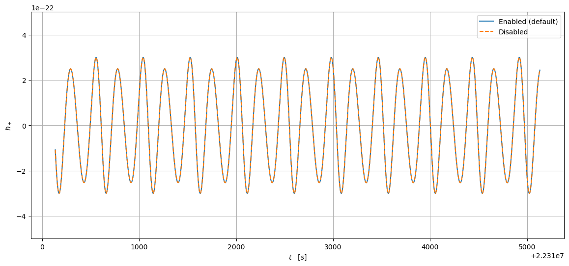
The 1PA contributions to the amplitudes and the evolution of the primary mass and spin can both be disabled in the waveform generator using suitable keyword arguments when instantiating the generator:

waveform_generator_off = GenerateEMRIWaveform(
        "Circ1PAT1R",
        #sum_kwargs = dict(pad_output=True),
        inspiral_kwargs = {"evolve_primary": False},
        amplitude_kwargs = {"zero_PA_amps_only": True},
        frame = "detector"
    )
h_on = waveform_generator(*params, T=T, dt=dt)  #default behaviour
h_off = waveform_generator_off(*params, T=T, dt=dt)

plt.gcf().set_size_inches(14, 6)
plt.plot(dt*np.arange(len(h_on))[-5000:], h_on.real[-5000:], label="Enabled (default)")
plt.plot(dt*np.arange(len(h_off))[-5000:], h_off.real[-5000:], ls='--', label="Disabled")
plt.ylim(-5e-22, 5e-22)
plt.ylabel(r"$h_+$")
plt.xlabel(r"$t \quad [s]$")
plt.legend()
plt.grid()

plt.gcf().set_size_inches(14, 6)
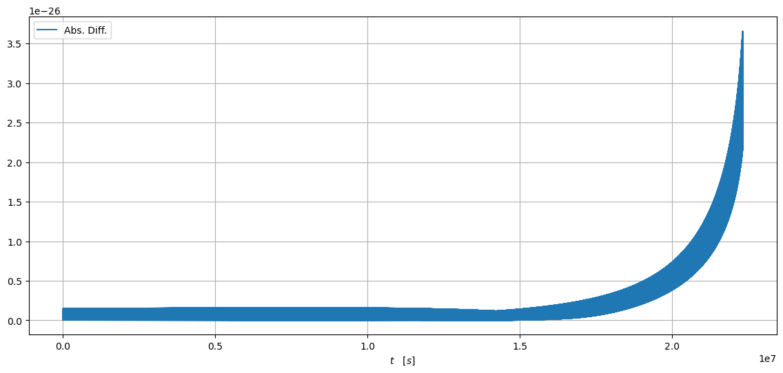
plt.plot(dt*np.arange(len(h_on)), np.abs(h_on - h_off), label="Abs. Diff.")
plt.legend(loc="upper left")
plt.xlabel(r"$t \quad [s]$")
plt.grid()